Quasars are among the most distant observable objects known in the universe – the furthest observed have exceeded redshifts of z = 7. Combined with their long lifetimes, quasars have the potential to be exceptional contributions to the cosmic distance ladder. Currently the distance ladder reaches only as far as type Ia supernovae can be observed (z ~ 1), but with the addition of quasars we could easily extend the distance ladder well beyond z = 2 and in principle past z = 7. At these redshifts we would be able to make next generation constraints on the cosmological parameters constraining the Hubble expansion and probe deeper into the ever prevalent Hubble tension.
The trouble however is that, unlike other rungs of the distance ladder such as Cepheid variables which all have the same luminosity, the quasar population ranges in luminosity over several orders of magnitude. Type Ia supernovea also had displayed a similar variation in luminosity over their population, but it was soon realized that a very tight relation was shared between the peak luminosity of the supernova and how quickly it dimmed in the days following its peak brightness. This relation allowed them to be standardized – that is to say, observing how quickly the supernova dims from its peak brightness one could immediately tell how bright the quasar really was. So in order to add quasars to the distance ladder we would need to find some relation of parameters in the light coming from the quasar that would allow us to determine with good precission the exact luminosity of the quasar. Once we determine how luminous the quasar should be we can relate it back to how luminous we observe it which gives us a measure of the distance to the quasar. There have been many attempts towards finding such a relation but most have been plagued by large dispersion making determination of the distance very inaccurate.
We have however noticed a tight relation between the variational rate of the quasar’s flux and its absolute magnitude. A quasar’s light curve varies rapidly with time. We are able to find the average rate or slope of these variations by fitting the light curve with many different sized windows.
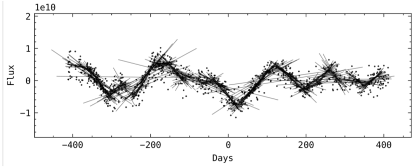
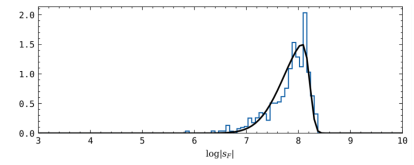
The variational rate is then just defined to be the most likely slope. More consistently we fit the population of slopes with a skewnorm distribution and we take the peak of the fit to determine a quasar’s variational rate.
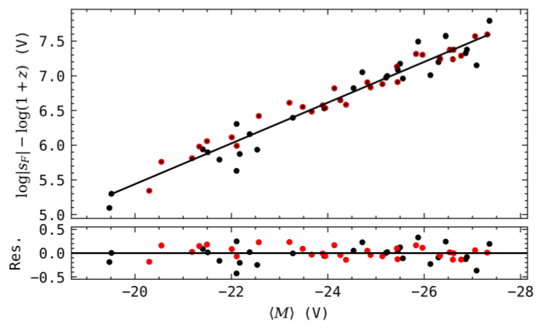
Repeating this for many quasars and plotting the variational rate versus the absolute magnitude of the quasar we find a tight correlation.
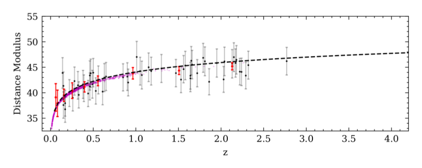
If this relation is a general feature of all quasars then we can use this to construct a Hubble diagram and constrain cosmological parameters. Shown below is such a Hubble diagram for the quasars from the MACHO survey along with the type Ia supernovae from the Pantheon survey (magenta). The quasars follow a LCDM cosmology (dashed line) with the Planck best fit parameters which is evident of our model dependent calibration method. With following work we will reduce our model dependence so that the behavior of quasars in our Hubble diagram will show the true expansion behavior.